| <!--Copyright 2023 The HuggingFace Team. All rights reserved. |
|
|
| Licensed under the Apache License, Version 2.0 (the "License"); you may not use this file except in compliance with |
| the License. You may obtain a copy of the License at |
|
|
| http://www.apache.org/licenses/LICENSE-2.0 |
|
|
| Unless required by applicable law or agreed to in writing, software distributed under the License is distributed on |
| an "AS IS" BASIS, WITHOUT WARRANTIES OR CONDITIONS OF ANY KIND, either express or implied. See the License for the |
| specific language governing permissions and limitations under the License. |
| --> |
|
|
| [[open-in-colab]] |
|
|
|
|
| # Diffusion 모델을 학습하기 |
|
|
| Unconditional 이미지 생성은 학습에 사용된 데이터셋과 유사한 이미지를 생성하는 diffusion 모델에서 인기 있는 어플리케이션입니다. 일반적으로, 가장 좋은 결과는 특정 데이터셋에 사전 훈련된 모델을 파인튜닝하는 것으로 얻을 수 있습니다. 이 [허브](https://huggingface.co/search/full-text?q=unconditional-image-generation&type=model)에서 이러한 많은 체크포인트를 찾을 수 있지만, 만약 마음에 드는 체크포인트를 찾지 못했다면, 언제든지 스스로 학습할 수 있습니다! |
|
|
| 이 튜토리얼은 나만의 🦋 나비 🦋를 생성하기 위해 [Smithsonian Butterflies](https://huggingface.co/datasets/huggan/smithsonian_butterflies_subset) 데이터셋의 하위 집합에서 [`UNet2DModel`] 모델을 학습하는 방법을 가르쳐줄 것입니다. |
|
|
| <Tip> |
|
|
| 💡 이 학습 튜토리얼은 [Training with 🧨 Diffusers](https://colab.research.google.com/github/huggingface/notebooks/blob/main/diffusers/training_example.ipynb) 노트북 기반으로 합니다. Diffusion 모델의 작동 방식 및 자세한 내용은 노트북을 확인하세요! |
|
|
| </Tip> |
|
|
| 시작 전에, 🤗 Datasets을 불러오고 전처리하기 위해 데이터셋이 설치되어 있는지 다수 GPU에서 학습을 간소화하기 위해 🤗 Accelerate 가 설치되어 있는지 확인하세요. 그 후 학습 메트릭을 시각화하기 위해 [TensorBoard](https://www.tensorflow.org/tensorboard)를 또한 설치하세요. (또한 학습 추적을 위해 [Weights & Biases](https://docs.wandb.ai/)를 사용할 수 있습니다.) |
|
|
| ```bash |
| !pip install diffusers[training] |
| ``` |
|
|
| 커뮤니티에 모델을 공유할 것을 권장하며, 이를 위해서 Hugging Face 계정에 로그인을 해야 합니다. (계정이 없다면 [여기](https://hf.co/join)에서 만들 수 있습니다.) 노트북에서 로그인할 수 있으며 메시지가 표시되면 토큰을 입력할 수 있습니다. |
|
|
| ```py |
| >>> from huggingface_hub import notebook_login |
| |
| >>> notebook_login() |
| ``` |
|
|
| 또는 터미널로 로그인할 수 있습니다: |
|
|
| ```bash |
| huggingface-cli login |
| ``` |
|
|
| 모델 체크포인트가 상당히 크기 때문에 [Git-LFS](https://git-lfs.com/)에서 대용량 파일의 버전 관리를 할 수 있습니다. |
|
|
| ```bash |
| !sudo apt -qq install git-lfs |
| !git config --global credential.helper store |
| ``` |
|
|
|
|
| ## 학습 구성 |
|
|
| 편의를 위해 학습 파라미터들을 포함한 `TrainingConfig` 클래스를 생성합니다 (자유롭게 조정 가능): |
|
|
| ```py |
| >>> from dataclasses import dataclass |
| |
| |
| >>> @dataclass |
| ... class TrainingConfig: |
| ... image_size = 128 # 생성되는 이미지 해상도 |
| ... train_batch_size = 16 |
| ... eval_batch_size = 16 # 평가 동안에 샘플링할 이미지 수 |
| ... num_epochs = 50 |
| ... gradient_accumulation_steps = 1 |
| ... learning_rate = 1e-4 |
| ... lr_warmup_steps = 500 |
| ... save_image_epochs = 10 |
| ... save_model_epochs = 30 |
| ... mixed_precision = "fp16" # `no`는 float32, 자동 혼합 정밀도를 위한 `fp16` |
| ... output_dir = "ddpm-butterflies-128" # 로컬 및 HF Hub에 저장되는 모델명 |
| |
| ... push_to_hub = True # 저장된 모델을 HF Hub에 업로드할지 여부 |
| ... hub_private_repo = False |
| ... overwrite_output_dir = True # 노트북을 다시 실행할 때 이전 모델에 덮어씌울지 |
| ... seed = 0 |
| |
| |
| >>> config = TrainingConfig() |
| ``` |
|
|
|
|
| ## 데이터셋 불러오기 |
|
|
| 🤗 Datasets 라이브러리와 [Smithsonian Butterflies](https://huggingface.co/datasets/huggan/smithsonian_butterflies_subset) 데이터셋을 쉽게 불러올 수 있습니다. |
|
|
| ```py |
| >>> from datasets import load_dataset |
| |
| >>> config.dataset_name = "huggan/smithsonian_butterflies_subset" |
| >>> dataset = load_dataset(config.dataset_name, split="train") |
| ``` |
|
|
| 💡[HugGan Community Event](https://huggingface.co/huggan) 에서 추가의 데이터셋을 찾거나 로컬의 [`ImageFolder`](https://huggingface.co/docs/datasets/image_dataset#imagefolder)를 만듦으로써 나만의 데이터셋을 사용할 수 있습니다. HugGan Community Event 에 가져온 데이터셋의 경우 레포지토리의 id로 `config.dataset_name` 을 설정하고, 나만의 이미지를 사용하는 경우 `imagefolder` 를 설정합니다. |
|
|
| 🤗 Datasets은 [`~datasets.Image`] 기능을 사용해 자동으로 이미지 데이터를 디코딩하고 [`PIL.Image`](https://pillow.readthedocs.io/en/stable/reference/Image.html)로 불러옵니다. 이를 시각화 해보면: |
|
|
| ```py |
| >>> import matplotlib.pyplot as plt |
| |
| >>> fig, axs = plt.subplots(1, 4, figsize=(16, 4)) |
| >>> for i, image in enumerate(dataset[:4]["image"]): |
| ... axs[i].imshow(image) |
| ... axs[i].set_axis_off() |
| >>> fig.show() |
| ``` |
|
|
|  |
|
|
| 이미지는 모두 다른 사이즈이기 때문에, 우선 전처리가 필요합니다: |
|
|
| - `Resize` 는 `config.image_size` 에 정의된 이미지 사이즈로 변경합니다. |
| - `RandomHorizontalFlip` 은 랜덤적으로 이미지를 미러링하여 데이터셋을 보강합니다. |
| - `Normalize` 는 모델이 예상하는 [-1, 1] 범위로 픽셀 값을 재조정 하는데 중요합니다. |
|
|
| ```py |
| >>> from torchvision import transforms |
| |
| >>> preprocess = transforms.Compose( |
| ... [ |
| ... transforms.Resize((config.image_size, config.image_size)), |
| ... transforms.RandomHorizontalFlip(), |
| ... transforms.ToTensor(), |
| ... transforms.Normalize([0.5], [0.5]), |
| ... ] |
| ... ) |
| ``` |
|
|
| 학습 도중에 `preprocess` 함수를 적용하려면 🤗 Datasets의 [`~datasets.Dataset.set_transform`] 방법이 사용됩니다. |
|
|
| ```py |
| >>> def transform(examples): |
| ... images = [preprocess(image.convert("RGB")) for image in examples["image"]] |
| ... return {"images": images} |
| |
| |
| >>> dataset.set_transform(transform) |
| ``` |
|
|
| 이미지의 크기가 조정되었는지 확인하기 위해 이미지를 다시 시각화해보세요. 이제 [DataLoader](https://pytorch.org/docs/stable/data#torch.utils.data.DataLoader)에 데이터셋을 포함해 학습할 준비가 되었습니다! |
|
|
| ```py |
| >>> import torch |
| |
| >>> train_dataloader = torch.utils.data.DataLoader(dataset, batch_size=config.train_batch_size, shuffle=True) |
| ``` |
|
|
|
|
| ## UNet2DModel 생성하기 |
|
|
| 🧨 Diffusers에 사전학습된 모델들은 모델 클래스에서 원하는 파라미터로 쉽게 생성할 수 있습니다. 예를 들어, [`UNet2DModel`]를 생성하려면: |
|
|
| ```py |
| >>> from diffusers import UNet2DModel |
| |
| >>> model = UNet2DModel( |
| ... sample_size=config.image_size, # 타겟 이미지 해상도 |
| ... in_channels=3, # 입력 채널 수, RGB 이미지에서 3 |
| ... out_channels=3, # 출력 채널 수 |
| ... layers_per_block=2, # UNet 블럭당 몇 개의 ResNet 레이어가 사용되는지 |
| ... block_out_channels=(128, 128, 256, 256, 512, 512), # 각 UNet 블럭을 위한 출력 채널 수 |
| ... down_block_types=( |
| ... "DownBlock2D", # 일반적인 ResNet 다운샘플링 블럭 |
| ... "DownBlock2D", |
| ... "DownBlock2D", |
| ... "DownBlock2D", |
| ... "AttnDownBlock2D", # spatial self-attention이 포함된 일반적인 ResNet 다운샘플링 블럭 |
| ... "DownBlock2D", |
| ... ), |
| ... up_block_types=( |
| ... "UpBlock2D", # 일반적인 ResNet 업샘플링 블럭 |
| ... "AttnUpBlock2D", # spatial self-attention이 포함된 일반적인 ResNet 업샘플링 블럭 |
| ... "UpBlock2D", |
| ... "UpBlock2D", |
| ... "UpBlock2D", |
| ... "UpBlock2D", |
| ... ), |
| ... ) |
| ``` |
|
|
| 샘플의 이미지 크기와 모델 출력 크기가 맞는지 빠르게 확인하기 위한 좋은 아이디어가 있습니다: |
|
|
| ```py |
| >>> sample_image = dataset[0]["images"].unsqueeze(0) |
| >>> print("Input shape:", sample_image.shape) |
| Input shape: torch.Size([1, 3, 128, 128]) |
| |
| >>> print("Output shape:", model(sample_image, timestep=0).sample.shape) |
| Output shape: torch.Size([1, 3, 128, 128]) |
| ``` |
|
|
| 훌륭해요! 다음, 이미지에 약간의 노이즈를 더하기 위해 스케줄러가 필요합니다. |
|
|
|
|
| ## 스케줄러 생성하기 |
|
|
| 스케줄러는 모델을 학습 또는 추론에 사용하는지에 따라 다르게 작동합니다. 추론시에, 스케줄러는 노이즈로부터 이미지를 생성합니다. 학습시 스케줄러는 diffusion 과정에서의 특정 포인트로부터 모델의 출력 또는 샘플을 가져와 *노이즈 스케줄* 과 *업데이트 규칙*에 따라 이미지에 노이즈를 적용합니다. |
|
|
| `DDPMScheduler`를 보면 이전으로부터 `sample_image`에 랜덤한 노이즈를 더하는 `add_noise` 메서드를 사용합니다: |
|
|
| ```py |
| >>> import torch |
| >>> from PIL import Image |
| >>> from diffusers import DDPMScheduler |
| |
| >>> noise_scheduler = DDPMScheduler(num_train_timesteps=1000) |
| >>> noise = torch.randn(sample_image.shape) |
| >>> timesteps = torch.LongTensor([50]) |
| >>> noisy_image = noise_scheduler.add_noise(sample_image, noise, timesteps) |
| |
| >>> Image.fromarray(((noisy_image.permute(0, 2, 3, 1) + 1.0) * 127.5).type(torch.uint8).numpy()[0]) |
| ``` |
|
|
|  |
|
|
| 모델의 학습 목적은 이미지에 더해진 노이즈를 예측하는 것입니다. 이 단계에서 손실은 다음과 같이 계산될 수 있습니다: |
|
|
| ```py |
| >>> import torch.nn.functional as F |
| |
| >>> noise_pred = model(noisy_image, timesteps).sample |
| >>> loss = F.mse_loss(noise_pred, noise) |
| ``` |
|
|
| ## 모델 학습하기 |
|
|
| 지금까지, 모델 학습을 시작하기 위해 많은 부분을 갖추었으며 이제 남은 것은 모든 것을 조합하는 것입니다. |
|
|
| 우선 옵티마이저(optimizer)와 학습률 스케줄러(learning rate scheduler)가 필요할 것입니다: |
|
|
| ```py |
| >>> from diffusers.optimization import get_cosine_schedule_with_warmup |
| |
| >>> optimizer = torch.optim.AdamW(model.parameters(), lr=config.learning_rate) |
| >>> lr_scheduler = get_cosine_schedule_with_warmup( |
| ... optimizer=optimizer, |
| ... num_warmup_steps=config.lr_warmup_steps, |
| ... num_training_steps=(len(train_dataloader) * config.num_epochs), |
| ... ) |
| ``` |
|
|
| 그 후, 모델을 평가하는 방법이 필요합니다. 평가를 위해, `DDPMPipeline`을 사용해 배치의 이미지 샘플들을 생성하고 그리드 형태로 저장할 수 있습니다: |
|
|
| ```py |
| >>> from diffusers import DDPMPipeline |
| >>> import math |
| >>> import os |
| |
| |
| >>> def make_grid(images, rows, cols): |
| ... w, h = images[0].size |
| ... grid = Image.new("RGB", size=(cols * w, rows * h)) |
| ... for i, image in enumerate(images): |
| ... grid.paste(image, box=(i % cols * w, i // cols * h)) |
| ... return grid |
| |
| |
| >>> def evaluate(config, epoch, pipeline): |
| ... # 랜덤한 노이즈로 부터 이미지를 추출합니다.(이는 역전파 diffusion 과정입니다.) |
| ... # 기본 파이프라인 출력 형태는 `List[PIL.Image]` 입니다. |
| ... images = pipeline( |
| ... batch_size=config.eval_batch_size, |
| ... generator=torch.manual_seed(config.seed), |
| ... ).images |
| |
| ... # 이미지들을 그리드로 만들어줍니다. |
| ... image_grid = make_grid(images, rows=4, cols=4) |
| |
| ... # 이미지들을 저장합니다. |
| ... test_dir = os.path.join(config.output_dir, "samples") |
| ... os.makedirs(test_dir, exist_ok=True) |
| ... image_grid.save(f"{test_dir}/{epoch:04d}.png") |
| ``` |
|
|
| TensorBoard에 로깅, 그래디언트 누적 및 혼합 정밀도 학습을 쉽게 수행하기 위해 🤗 Accelerate를 학습 루프에 함께 앞서 말한 모든 구성 정보들을 묶어 진행할 수 있습니다. 허브에 모델을 업로드 하기 위해 레포지토리 이름 및 정보를 가져오기 위한 함수를 작성하고 허브에 업로드할 수 있습니다. |
|
|
| 💡아래의 학습 루프는 어렵고 길어 보일 수 있지만, 나중에 한 줄의 코드로 학습을 한다면 그만한 가치가 있을 것입니다! 만약 기다리지 못하고 이미지를 생성하고 싶다면, 아래 코드를 자유롭게 붙여넣고 작동시키면 됩니다. 🤗 |
|
|
| ```py |
| >>> from accelerate import Accelerator |
| >>> from huggingface_hub import HfFolder, Repository, whoami |
| >>> from tqdm.auto import tqdm |
| >>> from pathlib import Path |
| >>> import os |
| |
| |
| >>> def get_full_repo_name(model_id: str, organization: str = None, token: str = None): |
| ... if token is None: |
| ... token = HfFolder.get_token() |
| ... if organization is None: |
| ... username = whoami(token)["name"] |
| ... return f"{username}/{model_id}" |
| ... else: |
| ... return f"{organization}/{model_id}" |
| |
| |
| >>> def train_loop(config, model, noise_scheduler, optimizer, train_dataloader, lr_scheduler): |
| ... # accelerator와 tensorboard 로깅 초기화 |
| ... accelerator = Accelerator( |
| ... mixed_precision=config.mixed_precision, |
| ... gradient_accumulation_steps=config.gradient_accumulation_steps, |
| ... log_with="tensorboard", |
| ... logging_dir=os.path.join(config.output_dir, "logs"), |
| ... ) |
| ... if accelerator.is_main_process: |
| ... if config.push_to_hub: |
| ... repo_name = get_full_repo_name(Path(config.output_dir).name) |
| ... repo = Repository(config.output_dir, clone_from=repo_name) |
| ... elif config.output_dir is not None: |
| ... os.makedirs(config.output_dir, exist_ok=True) |
| ... accelerator.init_trackers("train_example") |
| |
| ... # 모든 것이 준비되었습니다. |
| ... # 기억해야 할 특정한 순서는 없으며 준비한 방법에 제공한 것과 동일한 순서로 객체의 압축을 풀면 됩니다. |
| ... model, optimizer, train_dataloader, lr_scheduler = accelerator.prepare( |
| ... model, optimizer, train_dataloader, lr_scheduler |
| ... ) |
| |
| ... global_step = 0 |
| |
| ... # 이제 모델을 학습합니다. |
| ... for epoch in range(config.num_epochs): |
| ... progress_bar = tqdm(total=len(train_dataloader), disable=not accelerator.is_local_main_process) |
| ... progress_bar.set_description(f"Epoch {epoch}") |
| |
| ... for step, batch in enumerate(train_dataloader): |
| ... clean_images = batch["images"] |
| ... # 이미지에 더할 노이즈를 샘플링합니다. |
| ... noise = torch.randn(clean_images.shape).to(clean_images.device) |
| ... bs = clean_images.shape[0] |
| |
| ... # 각 이미지를 위한 랜덤한 타임스텝(timestep)을 샘플링합니다. |
| ... timesteps = torch.randint( |
| ... 0, noise_scheduler.config.num_train_timesteps, (bs,), device=clean_images.device |
| ... ).long() |
| |
| ... # 각 타임스텝의 노이즈 크기에 따라 깨끗한 이미지에 노이즈를 추가합니다. |
| ... # (이는 foward diffusion 과정입니다.) |
| ... noisy_images = noise_scheduler.add_noise(clean_images, noise, timesteps) |
| |
| ... with accelerator.accumulate(model): |
| ... # 노이즈를 반복적으로 예측합니다. |
| ... noise_pred = model(noisy_images, timesteps, return_dict=False)[0] |
| ... loss = F.mse_loss(noise_pred, noise) |
| ... accelerator.backward(loss) |
| |
| ... accelerator.clip_grad_norm_(model.parameters(), 1.0) |
| ... optimizer.step() |
| ... lr_scheduler.step() |
| ... optimizer.zero_grad() |
| |
| ... progress_bar.update(1) |
| ... logs = {"loss": loss.detach().item(), "lr": lr_scheduler.get_last_lr()[0], "step": global_step} |
| ... progress_bar.set_postfix(**logs) |
| ... accelerator.log(logs, step=global_step) |
| ... global_step += 1 |
| |
| ... # 각 에포크가 끝난 후 evaluate()와 몇 가지 데모 이미지를 선택적으로 샘플링하고 모델을 저장합니다. |
| ... if accelerator.is_main_process: |
| ... pipeline = DDPMPipeline(unet=accelerator.unwrap_model(model), scheduler=noise_scheduler) |
| |
| ... if (epoch + 1) % config.save_image_epochs == 0 or epoch == config.num_epochs - 1: |
| ... evaluate(config, epoch, pipeline) |
| |
| ... if (epoch + 1) % config.save_model_epochs == 0 or epoch == config.num_epochs - 1: |
| ... if config.push_to_hub: |
| ... repo.push_to_hub(commit_message=f"Epoch {epoch}", blocking=True) |
| ... else: |
| ... pipeline.save_pretrained(config.output_dir) |
| ``` |
|
|
| 휴, 코드가 꽤 많았네요! 하지만 🤗 Accelerate의 [`~accelerate.notebook_launcher`] 함수와 학습을 시작할 준비가 되었습니다. 함수에 학습 루프, 모든 학습 인수, 학습에 사용할 프로세스 수(사용 가능한 GPU의 수를 변경할 수 있음)를 전달합니다: |
|
|
| ```py |
| >>> from accelerate import notebook_launcher |
| |
| >>> args = (config, model, noise_scheduler, optimizer, train_dataloader, lr_scheduler) |
| |
| >>> notebook_launcher(train_loop, args, num_processes=1) |
| ``` |
|
|
| 한번 학습이 완료되면, diffusion 모델로 생성된 최종 🦋이미지🦋를 확인해보길 바랍니다! |
|
|
| ```py |
| >>> import glob |
| |
| >>> sample_images = sorted(glob.glob(f"{config.output_dir}/samples/*.png")) |
| >>> Image.open(sample_images[-1]) |
| ``` |
|
|
| 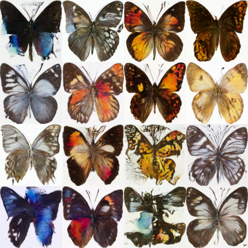 |
|
|
| ## 다음 단계 |
|
|
| Unconditional 이미지 생성은 학습될 수 있는 작업 중 하나의 예시입니다. 다른 작업과 학습 방법은 [🧨 Diffusers 학습 예시](../training/overview) 페이지에서 확인할 수 있습니다. 다음은 학습할 수 있는 몇 가지 예시입니다: |
|
|
| - [Textual Inversion](../training/text_inversion), 특정 시각적 개념을 학습시켜 생성된 이미지에 통합시키는 알고리즘입니다. |
| - [DreamBooth](../training/dreambooth), 주제에 대한 몇 가지 입력 이미지들이 주어지면 주제에 대한 개인화된 이미지를 생성하기 위한 기술입니다. |
| - [Guide](../training/text2image) 데이터셋에 Stable Diffusion 모델을 파인튜닝하는 방법입니다. |
| - [Guide](../training/lora) LoRA를 사용해 매우 큰 모델을 빠르게 파인튜닝하기 위한 메모리 효율적인 기술입니다. |
|
|
